A fundamental goal for many people, explicit or otherwise, is to be maximally happy. Easily said, not always so easily done. So how might we set about raising our level of happiness? OK, at some level, we’re all individuals with our own set of wishes and desires. But, at a more macro level, there are underlying patterns in many human attributes that lead me to believe that learning what typically makes other people happy might be useful with regards to understanding what may help maintain or improve our own happiness.
With that in mind, let’s see if we can pursue a data driven answer to this question: what should our priorities or behaviours likely be if we want to optimise for happiness?
For a data driven answer, we’re going to need some data. I settled on the freely available HappyDB corpus (thanks, researchers!).
The corpus contains around 100,000 free text answers, crowdsourced from members of the public who had signed up to Mechanical Turk, to this question:
What made you happy today? Reflect on the past {24 hours|3 months}, and recall three actual events that happened to you that made you happy. Write down your happy moment in a complete sentence.
Write three such moments.
Examples of happy moments we are NOT looking for (e.g events in distant past, partial sentence):
– The day I married my spouse
– My Dog
It should be noted that the average Mechanical Turk user is not representative of the average person in the world and hence any findings may have limited generalisability. However, the file does contain some demographics which we consider digging into later in case there’s any correspondence between one’s personal characteristics and what makes them happy. Perhaps most notably, around 86% of respondents were from the USA, so there will clearly be a geographic / cultural bias at play. However, being from the UK, a similarly “westernised country”, this may be less of a problem for me if I personally wish to act on the results. A more varied geographical or cultural comparison on drivers of happiness would however be a fascinating exercise.
I’m most interested in eliciting the potential drivers of happiness in a manner conducive to informing my mid-to-longer term goals. With that in mind, here I’m only looking at the longer term variant of the question – what made people happy in the past 3 months? A followup could certainly be whether or not the same type of things that people report having made them happy over a 3 month timeframe correspond to the things that people report making them happy on a day-to-day basis.
So, having downloaded the dataset , the first step is to read it into our analysis software. Here I will be using R. The researchers supply several few data files, which are described on their Github page. Here I decided to use the file where they’d generously cleaned up a few of the less valid looking entries, for instance if they were blank, had only a single word, or seemed to be misspelled, called “cleaned_hm.csv“.
Whilst some metadata is also included in that file, for the first part of this exercise I am only interested in these columns:
- hmid: the unique ID number for the “happy moment”
- wmid: an ID number that tells us which “worker” i.e. respondent answered the question. One person may have responded to the question several times. It’s also a way to link up the demographic attributes of the respondent in future if we want to.
- cleaned_hm: the actual (cleaned up) text of the response the user gave to the happiness question
We’ll also use the “reflection_period” field to filter down to only the responses to the 3 month version of the question. This field contains “3m” in the row for these 3-month responses.
library(readr)
library(dplyr)

happy_db <- read_csv(".\\happy_db_data\\rit-public-HappyDB-b9e529e\\happydb\\data\\cleaned_hm.csv")

happy_data <- filter(happy_db, reflection_period == "3m") %>%
select(hmid, wid, cleaned_hm)
Let’s take a look at a few rows of the data to ensure everything’s looking OK.
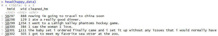
OK, that looks good, and perhaps already gives us a little preview of what sort of things make people happy,
Checking the recordcount – nrow(happy_data) – shows we have 50,704 happy moments to look at after the filters have been applied. Reading them all one by one isn’t going to be much fun, so let’s load up some text analysis tools!
First, I wanted to tokenise the text. That is to say, extract each individual word from the each response to the happiness question and put it onto its own row. This makes certain types of data cleaning and analysis way easier, especially if, like me, you’re a tidyverse advocate. I may want to be able to reconstruct the tokenised sentences in future, so will keep track of which word comes from which happy moment, by logging the relevant happy moment ID, “hmid”, on each row.
Past experience (and common sense) tells me that some types of words may be more interesting to analyse than others. I won’t learn a lot from knowing how many respondents used the word “and”.
One approach could be to classify words as to their “part of speech” type – adjectives, verbs, nouns and so on. My intuition is that people’s happiness might be influenced by encountering certain objects (in the widest possible sense – awkwardly incorporating people into that classification) or engaging in specific activities. This feels like a potential close fit to the nouns and verb speech parts. So let’s begin by extracting each word and classifying it as to whether it’s a noun, verb or something else.
One R option for this is the cleanNLP library. cleanNLP includes functions to tokenise and “annotate” each word with respect to what part of speech it is. It can actually use a variety of natural language processing backends to do this, some more fancy than others. Some require installing non-R software like Python or Java, which, to keep it simple here, I’m going to avoid. So I’m going to use the udpipe library, which is pure R, and hence can be installed with the standard install.packages(“udpipe”) command if necessary.
Once cleanNLP is installed, we need to ask it to split up and tag our text as to whether each word is a noun, verb and so on. First we initialise the backend we want to use, udpipe. Then we use the cnlp_annotate command to perform the tokenisation and annotation, passing it:
- the name of the dataframe containing the question responses: happy_data.
- the name of the field which contains the actual text of the responses, as text_var.
- the name of the field that identifies each individual unique response as doc_var.
This process can take a long time to complete, so don’t start it if you’re in a hurry.
Finally, we’ll take the resulting “annotation” object and extract the table of annotated words (aka tokens) from it, to make it easy to analyse with standard tidy tools.
install.packages("cleanNLP")
library(cleanNLP)

# initialise udpipe annotation engine

cnlp_init_udpipe()

# annotate text

happy_data_annotated <- cnlp_annotate(happy_data, as_strings = TRUE,
                                   text_var = "cleaned_hm", doc_var = "hmid")

# extract tokens into a data frame

happy_terms <- happy_data_annotated %>%
  cnlp_get_token()
OK, let’s see what we have, comparing this output to the original response data for the first entry.
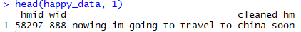
After:

Lovely. In our annotated token data, we can see the id field matches the hmid field of the response file, allowing us to keep track of which words came from which response.
Each word of the response is now a row, in the field “word”. Furthermore, the word has also been converted to its lemma in the lemma field – a lemma being the base “dictionary” version of the word – for instance the words “studying” and “studies” both have the lemma “study“. This lemmatisation seems useful if I’m interested in a general overview of the subjects people mention in response to the happiness question, insomuch as it may group words together that have the same basic meaning.
Of course it can’t always be perfect – the above example in fact has a type of error, in that the word “nowing” has been lemmatised as “now”, whereas one has to assume the respondent actually meant “knowing”, with a lemma more like “know”. However, this is user error – they misspelt their response. I don’t fancy going through each response to fix up these types of errors, so for the purposes of this quick analysis I’ll just assume them to be relatively rare.
We can also see the in the field “upos” that the words have been classified into their grammatical function – including the verbs and nouns we’re looking for. upos stands for “universal part of speech”, and you can see what the abbreviations mean here.
The “pos” field divides these categories up further, and can be deciphered as being Penn part of speech tags. In the above example, you can see some verbs are categorised as VBG and others as VB. This is distinguishing between the base form of a verb and its present participle. I’m not going to concern myself with these differences, so will stick to the upos field.
Now we have this more usable format, there’s still a little more data cleansing I want to do.
- One part of speech (hereafter “POS”) category is called PUNCT, meaning punctuation. I don’t really want to include punctuation marks in my analysis, so will remove any words that are classified as PUNCT.
- Same goes for the category SYM, which are symbols.
- I also want to remove stopwords. These are words like “the”, “a” and other very common words that are typically not too informative when it comes to analysing sentences at a per-word level. Here I used the snowball list to define which words are in that category. This list is included in the excellent tidytext package, the usage of which is documented in its companion book.
- I’m also going to remove words that directly correspond to “happy”. Given the question itself is “what makes you happy?” I feel safe to assume that all the responses should relate to happiness. Knowing people used the word “happy” a lot won’t add much to my understanding.
Here’s how I did it:
happy_terms <- filter(happy_terms, upos != "PUNCT" & upos != "SYM") %>%
  anti_join(filter(stop_words, lexicon == "snowball"), by = c("lemma" = "word")) %>%
  filter(!(lemma %in% c("happy", "happiness", "happier")))
OK, now we have a nice cleanish list of the dictionary words from the responses. Let’s take a look at what they are! We’ll start with the most obvious type of analysis, a frequency count. What are the most common words people used in their responses?
Let’s start with “things”, i.e. nouns. Here are the top 20 nouns used in the answers to the happiness question.
library(ggplot2)

filter(happy_terms, upos == "NOUN") %>%
  count(lemma, sort = TRUE) %>%
  arrange(desc(n)) %>%
  slice(1:20) %>%
  ggplot(aes(x = reorder(lemma, n, mean), y = n)) +
  geom_col() +
  coord_flip() +
  theme_bw() +
  labs(title = "Most common nouns in responses to happiness question", x = "", y = "Count")

OK, there’s already some strong themes emerging there! Many nouns relate to people (friend, family, etc.), there’s a mention of jobs, and some more “occasion” based terms like birthday, event etc.
There’s also a lot of time frame indicators. Whilst it may eventually be interesting that there are more mentions of day than month, and more month mentions than year, for a simple first pass I’m not sure they add a lot. Let’s exclude them, and plot a larger sample of nouns. This time we’ll use a word cloud, where the size of the words are relative to the frequency of usage. Larger words are those that are used more often in the responses. For this, we can use the appropriately named library “wordcloud“.
It should be noted that, whilst wordclouds are more visually appealing than bar charts to many people, they are certainly harder to interpret in a precise way. However, here I’m more looking for the major themes, so I’ll live with that and go with the prettier option.
install.packages("wordcloud")
library(wordcloud)

# create a count of nouns, excluding some time based ones

happy_token_frequency_nlp_noun <-
  filter(happy_terms, upos == "NOUN" & !(lemma %in% c("day", "time", "month", "week", "year", "today"))) %>%
  count(lemma, sort = TRUE)

# open a png graphics device so wordcloud gets saved to disk as a png

png("wordcloud_packages.png", width=12,height=8, units='in', res=300)

# create the wordcloud

wordcloud(words = happy_token_frequency_nlp_noun$lemma, freq = happy_token_frequency_nlp_noun$n, max.words = 150, colors = c("grey60", "darkgoldenrod1", "tomato"))

# close the png device

dev.off()
A wordcloud of happy nouns:
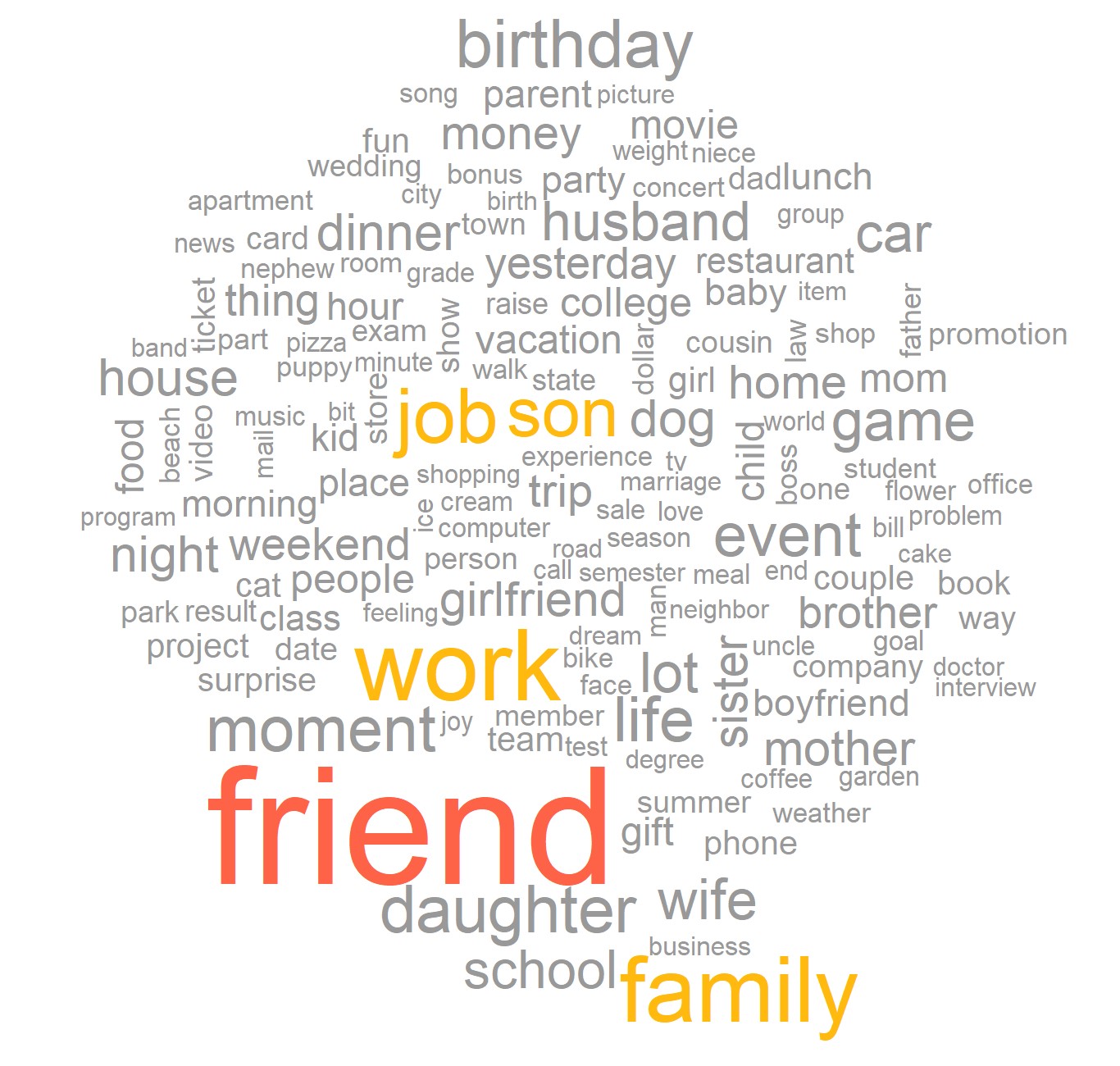
A cornucopia of happiness-inducing things! In this format, some commonalities truly stand out. It seems that friends make people particularly happy. Families are key too, although the number of times “family” is directly mentioned is lower than “friend”. That said, parts of family-esque structures such as son, daughter, wife, husband, girlfriend and boyfriend are also specifically mentioned with relatively high frequency. Basically, people are made happy by other people. Or even by our furry relatives – dog and cat are both in there.
Next most common, perhaps less intuitively, are words around what is probably employment – job and work.
There’s plenty of potentially “event” type words in there – event itself, but also birthday, date, dinner, game, movie et al. Perhaps these show what type of occasions are most associated with happy times. I can’t help but note that many of them sound again like opportunities for socialising.
There’s a few actual “things” in the more conventional sense too; insentient objects that you could own. They’re less prevalent in terms of mentions of any individual one, but car, computer, bike and phone some relevant examples that appear.
And then some perhaps less controllable phenomena – weather, season and surprise.
It must be noted these interpretations have to rely on assumptions based on preexisting knowledge of how people usually construct sentences and the norms for answering questions. We’re looking at single words in isolation. There’s no context.
If people are actually writing “Everything except my friend made me happy” then the word “friend” would still appear in the wordcloud. Intuitively though, this seems unlikely to be the main driver of it featuring so strongly. We may however dig deeper into context later. For now, we can also increase our confidence in the most straightforward interpretation by noting that there’s a fair bit of external research out there that suggests a positive connection between friendship and happiness, and even health, that would support these results. Happify produced a nice infographic summarising the results of a few such studies.
Next up, let’s repeat the exercise using verbs, or as I vaguely recall learning at primary school, “doing words”. What kind of actions do people take that results in them having a happy memory?
The code is very similar to the nouns example. Firstly, let’s filter and plot the most common verbs we found in the responses.
filter(happy_terms, upos == "VERB") %>%
  count(lemma, sort = TRUE) %>%
  arrange(desc(n)) %>%
  slice(1:20) %>%
  ggplot(aes(x = reorder(lemma, n, mean), y = n)) +
  geom_col() +
  coord_flip() +
  theme_bw() +
  labs(title = "Most common verbs in responses to happiness question", x = "", y = "Count")
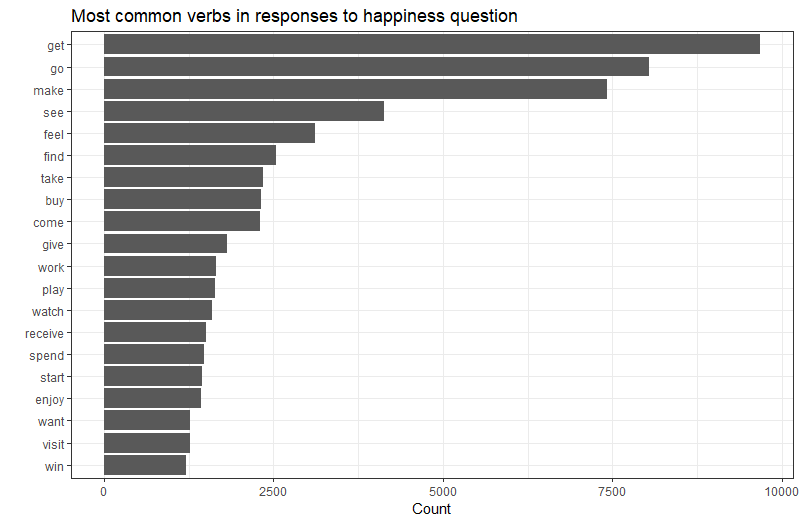
The top 3 there – get, go and make – seem be particularly prevalent compared to the rest. Getting things, going to places and the satisfaction of creating things are all things we might intuit are pleasing to the average human. However they’re somewhat vague, which makes me curious as to how exactly they’re being used in sentences. Are there particular things that show up as being got, gone to or made that generate happy memories?
To understand that, we’re going to have look at a bit of, at least simplistic, context. We’ll start by looking at the most common phrases those words appear in. To do this, we’ll use the tidytext library to generate “bigrams” – that is to say, each 2-word combination within the response sentences that those specific words are used in.
For example, if there’s a sentence ‘I love to make cakes’, then the bigrams involving ‘make’ here are:
- to make
- make cakes
If we calculate and count every such bigram, then, if enough people enjoy making cakes, that might pop out in our data.
First up though, remember that our analysis so far is actually showing the lemmas of the words used by the respondents, rather than the exact words themselves. So we’ll need to determine which words in our dataset are represented by the lemmas “get”, “go” and “make” in order to comprehensively find the appropriate bigrams in the text.
We can do that by looking for all the distinct combinations of lemma and word in our tokenised dataset. Here’s one way to see which unique real-world words in our dataset are represented by the lemma “get”:
filter(happy_terms, lemma == "get") %>%
  select(word) %>%
  mutate(word = tolower(word)) %>%
  distinct()

This means that we should look in the raw response text for any bigrams involving got, get, getting, gets or gotten if we want to see what the commonest contexts for the “get” responses are. To automate this a little, let’s create a vector for each of the 3 highly represented lemmas – get, go, and make – that include all the words that are grouped into that lemma.
get_words <- filter(happy_terms, lemma == "get") %>%
  select(word) %>%
  mutate(word = tolower(word)) %>%
  distinct() %>%
  pull(word)

go_words <- filter(happy_terms, lemma == "go") %>%
  select(word) %>%
  mutate(word = tolower(word)) %>%
    distinct() %>%
  pull(word)

make_words <- filter(happy_terms, lemma == "make") %>%
  select(word) %>%
  mutate(word = tolower(word)) %>%
    distinct() %>%
  pull(word)
The next step is to generate the bigrams themselves. Here I’m also removing the common, generally tedious, stopwords as we did before. This simplistic approach to stopwords does have some potentially problematic side-effects – including that if an interesting single word is surrounded entirely by stopwords then it will be excluded from this analysis. However, in terms of detecting a few interesting themes as opposed to creating a detailed linguistic analysis, I’m OK with that for now.
# create the bigrams

happy_bigrams <-  unnest_tokens(happy_data, bigram, cleaned_hm, token = "ngrams", n = 2) %>%
  separate(bigram, c("word1", "word2"), sep = " ") %>%
  filter(!(word1 %in% filter(stop_words, lexicon == "snowball")$word) & !(word2 %in% filter(stop_words, lexicon == "snowball")$word))

# create a count of how many time each bigram was found - sorting from most to least frequent

bigram_counts <- happy_bigrams %>%
  count(word1, word2, sort = TRUE)

# show the top 20 bigrams that use the 'get' lemma

filter(bigram_counts, word1 %in% get_words | word2 %in% get_words) %>%
    head(20) %>%
    ggplot(aes(x = reorder(paste(word1, word2), n, mean), y = n)) +
    geom_col() +
    coord_flip() +
    theme_bw() +
    labs(title = "Most common bigrams involving the 'get' lemma", x = "", y = "Count")
What do people like to get?
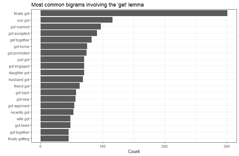
“finally got” may not tell us much about what was gotten, but evidently achieving something one has waited for for some time is particularly pleasing in this context. Other obvious themes there are mentions again of other people – son got, wife got, friend got, get together etc. Likewise there’s a few life events there – getting married, and work stuff like getting promoted or hired.
But my curiosity remains unabated. What sort of things are people happy that they “finally got”? To get some idea, I decided to split the responses up into five-word n-grams – think of these as being like bigrams, but looking at groups of 5 consecutive words rather than 2.
Groups of 5 words here will tend to produce low counts as people don’t necessarily express the same idea using precisely the same words – we may revisit this limitation in future! Nonetheless, it may give us a clue as to what some of the bigger topics are. We can use the unnest_tokens command from the tidytext library again. This is exactly what we did above to generate the bigrams, but this time specifying an n of 5, to specific that we want sequences of 5 words.
# make the 5-grams, keeping only those that were found at least twice
happy_fivegrams <-  unnest_tokens(happy_data, phrase, cleaned_hm, token = "ngrams", n = 5) %>%
  separate(phrase, c("word1", "word2", "word3", "word4", "word5"), sep = " ") %>%
  group_by(word1, word2, word3, word4, word5) %>%
  filter(n() >= 2 ) %>%
  ungroup()

# count how many times each 5-gram was used
fivegram_counts <- happy_fivegrams %>%
  count(word1, word2, word3, word4, word5, sort = TRUE)

 # show the top 15 that started with "finally got"
filter(fivegram_counts, word1 == "finally" & word2 == "got" ) %>%
   head(15)

Only a couple of people used most of the precise same phrases, but the most obvious feature that stands out here related to employment. People “finally” getting new jobs, or progressing towards the jobs they want, are occasions that make them happy.
Back now to drilling down into the common verb lemma bigrams: where are people going when they make happy memories?
# show the top 20 bigrams that use the 'go' lemma

filter(bigram_counts, word1 %in% go_words | word2 %in% go_words) %>%
    head(20) %>%
    ggplot(aes(x = reorder(paste(word1, word2), n, mean), y = n)) +
    geom_col() +
    coord_flip() +
    theme_bw() +
    labs(title = "Most common bigrams involving 'go' lemma", x = "", y = "Count")

Here, going shopping wins the frequency competition – although it’s certainly not usually an experience I personally enjoy! There’s a few references to family and friends again, and a predilection for going home. A couple of specific outdoor leisure activities – hiking and fishing – seem to suit some folk well. A less expected top 20 entry there was Pokemon Go, the “gotta-catch-em-all” augmented reality game, which, sure enough, does have the word “go” in its title. The human urge to collect apparently persists in the virtual world 🙂
Finally, what are people making that pleases them?
# show the top 20 bigrams that use the 'make' lemma

filter(bigram_counts, word1 %in% make_words | word2 %in% make_words) %>%
    head(20) %>%
    ggplot(aes(x = reorder(paste(word1, word2), n, mean), y = n)) +
    geom_col() +
    coord_flip() +
    theme_bw() +
    labs(title = "Most common bigrams involving 'make' lemma", x = "", y = "Count")
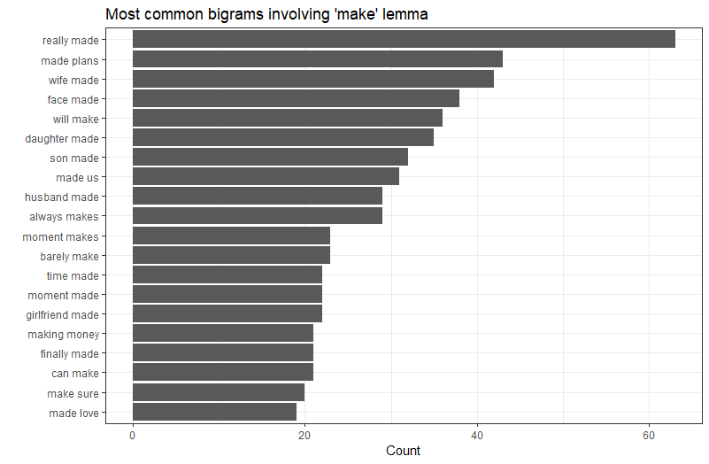
It’s not all about making in the sense of arts and crafts here. Making plans appeals to some – perhaps creating something that they can then look forward to occurring in the future. References to “moments” are pretty vague but perhaps describe happiness coming from specific events that could later be drilled down into.
There’s the ever-present social side of wives, sons, girlfriends et al featuring in the commonest bigrams. The hedonistic pleasures of money and sex also creep into the top 20.
OK, now we’ve dug a little into the 3 verb lemmas that dominate the most common verbs used, let’s take a look at the next most frequently used selection of verbs. Here again, we’ll use the (controversial) wordcloud, and hope it allows us to elucidate at least some common themes.
Removing “get”, “make” and “go” from the tokenised verb list, before wordclouding the most common of the remaining verb lemmas:
# filter the terms to show only verbs that are not get, make or go.

happy_token_frequency_nlp_verb_filtered <- filter(happy_terms, upos == "VERB" & !lemma %in% c("get", "make", "go")) %>%
count(lemma, sort = TRUE)

# open a png graphics device so wordcloud gets saved to disk as a png

png("wordcloud_verb_filtered.png", width=12,height=8, units='in', res=300)

# create the wordcloud

wordcloud(words = happy_token_frequency_nlp_verb_filtered$lemma, freq = happy_token_frequency_nlp_verb_filtered$n, max.words = 150, colors = c("grey60", "darkgoldenrod1", "tomato"))

# close the png device

dev.off()
A wordcloud of happy verbs:
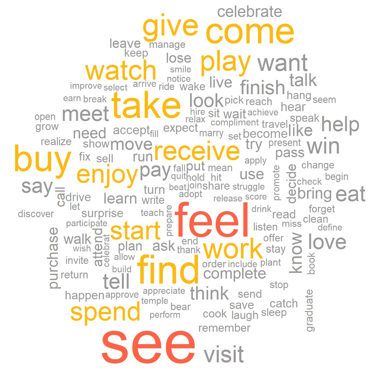
The highest volumes here are seen in experiential words – see and feel, vague as they might seem in this uni-word analysis. Perhaps though they hint towards the conclusions of some external research that suggests, at least after a certain point of privilege, people tend to gain more happiness from spending their money on experiences as opposed to objects.
Beyond that, some hints towards – suprise, surprise – social interactions appear. Give, receive, take, visit, love, meet, tell, say, play, talk, share, participate, listen, speak, invite and call, amongst other words, may all potentially fall into that category.
There’s “spend”, a further analysis of which could differentiate between whether we’re typically talking about spending time, spending money, or both. A hint towards the former existing at least to some extent is given by “buy” being a relatively common verb. “Work” also features, along with some almost-by-definition happiness inducers such as “win” and “celebrate”.
In terms of specific activities, we see hints at some intellectual pursuits: read, book, learn, know, graduate – together with some potentially fitness related activities: walk, run and move. Per the famous saying, eating and drinking also makes some people merry.
So, in conclusion:
That’s the end of our first step here, essentially variations on a frequency analysis of the words used by respondents when they’re asked to recall what made them happy in the past 3 months. Did it produce any insights?
My main takeaway here is really the key criticality of the social. Happiness seekers should usually prioritise people, where there’s an option to do so.
Yes, shopping, cars and phones and a few other inanimate objects of potential desire popped up. We also saw a few recreational activities that may or may not be social. Here I’m thinking of walking, running, fishing and hiking. It’s perhaps also notable that those examples happen to be potentially physically active activities that often take place outside. There’s external research extolling the well-being benefits of both being outdoors and physical exercise.
Words associated with education, learning and employment also appeared with relatively high frequency, so a focus on optimising those aspects of life might also be worthwhile for improving satisfaction.
But references to friends, family and occasions that may involve other people dominated the discourse. Thus, when making life plans, it’s probably wise to consider the social – meaningful interaction with real live human beings – as a particularly high priority.
In our noun analysis above, the word “friend” stuck out. Whilst as life goes on, and often gets busier, it can sometimes be hard to find time to focus on these wider relationships, there’s external evidence that placing high a value on friendship is associated with improved well-being – potentially even moreso than the variation in valuing family relationships.
These effects seem to associate with even the most dramatic measures of well-being, with several studies suggesting that people who maintain strong social relationships of any kind tend to be happier, healthier and even live longer.
