Analysing your 23andme genetic data in R part 2: exploring the traits associated with your genome

In part one of this mini-series, you heroically obtained and imported your 23andme raw genome data into R. Fun as that was, let’s see if we can learn something interesting from it.  After all, 23andme does automatically provide several genomic analysis reports, but – for many sensible reasons – it is certainly limited in what it can show when compared to the entire literature of this exciting field.

It would be tiresome for me to repeat all the caveats you can find in part one, and all over the more responsible parts of the internet. But do remember that in the grand scheme of things we likely know only somewhere between “nothing” and “a little” so far about the implications of most of the SNPs you imported into R in part one.

Whilst there are rare exceptions, for the most part it seems like many “interesting” real-world human traits are a product of many variations in different SNPs, each of which have a relatively tiny effect size. In these cases, if you happen to have a T somewhere rather than an A, it’s usually unlikely on its own to produce to any huge “real world” outcome you’d notice alone. Or if it does, we don’t necessarily know it yet. Or perhaps it could, but only if you have certain other bases in certain other positions, many of which 23andme may not report on – even if we knew which ones were critical. That was a long and meandering sentence which could be summarised as “things are complicated”.

Note also that 23andme do provide a disclaimer on the raw data, as follows:

This data has undergone a general quality review however only a subset of markers have been individually validated for accuracy. As such, the data from 23andMe’s Browse Raw Data feature is suitable only for research, educational, and informational use and not for medical or other use.

So, all in all, what follows should be treated as a fun-only investigation. You should first seek the services of genetic medical professionals, including the all-important genetic counsellor, if you have any real concerns about what you might find.

But, for the data thrill-seekers,  let’s start by finding some info as which genotypes at which SNPs are thought to have some potential association with a known trait. This is part of what 23andme does for you in their standard reporting. However, they have legal obligations and true experts working on this. I, on the other hand, recently read “Genetics for Dummies”, so tread carefully.

How do we find out about the associations between your SNP results and any subsequent phenotypes? The obvious place, especially if you’re interested in a particular trait, is the ever-growing published scientific literature on genetics. Being privileged enough to count amongst my good friends a scientist who actually published papers involving this subject, I started there. Here, for example, is Dr Kaitlin Roke’s paper: “Evaluating Changes in Omega-3 Fatty Acid Intake after Receiving Personal FADS1 Genetic Information: A Randomized Nutrigenetic Intervention“. Extra credit is also very much due to her for being kind enough to help me out with some background knowledge.

Part of that fascinating study involved explaining to members of the public what the implications of the differing alleles possible at a specific SNP, rs174537, were with regards to the levels of Omega 3 fatty acids typically found in a person’s body, and how well the relevant conversion process proceeds. This may have dietary implications in terms of how much the person concerned should focus on increasing the amount of omega-3 laden food they eat – although it would be remiss of me to fail to mention the good doctor’s general advice that mostly everyone needs to up their levels anyway!

Anyway, to quote from their wonderfully clear description of the implications of the studied SNP:

…the document provided a brief overview of the reported difference in omega-3 FA levels in relation to a common SNP in FADS1 (rs174537)…individuals who are homozygote GG allele carriers have been reported to have more EPA in their bodies and an increased ability to convert ALA into EPA and DHA while individuals with at least one copy of the minor allele (GT or TT) were shown to have less EPA in their bodies and a reduced ability to convert ALA into EPA and DHA

Awesome, so here we have a definitive explanation as to which SNP was examined, and what the implications of the various genotypes are (which I’ve bolded for your convenience).

In part 1 of this post, we already saw how to filter your R-based 23andme data to view your results for a specific SNP, right? If you already completed all those import steps, you can do the same, just switching in the rsid of interest:

library(dplyr)
filter(genome_data_test, rsid == "rs174537")

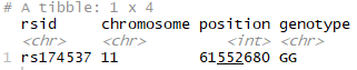
Run that, and if you are returned a result of either GT or TT then you’ll know you should be especially careful to ensure you are getting a good amount of omega 3 in your diet.

OK, this is super cool, but what if you don’t happen to know a friendly scientist, or don’t know what traits you’re particular interested in –  how might you evaluate the SNP implications at scale?

Whilst there’s no substitute for actual expertise, luckily there is a R library called “gwascat“, which enables you to access the  NHGRI-EBI Catalog of published genome-wide association studies via a data structure in R. It has a whole lot of info in it, descriptions of the fields you end up with mostly being shown here. The critical point is that it contains a list of SNPs, associated traits and relevant genotypes, together with the references to the publications that found the associations should you want to get more details.

The first thing to do is install gwascat. gwascat is a bioconductor package, rather than the business-user-typical cran packages. So if you’re not a bioconductor user, there’s a slightly different installation routine, which you can see here.

But essentially:

source("https://bioconductor.org/biocLite.R")
biocLite("gwascat")
library(gwascat)

This took a while to install for me, but can just be left to get on with itself.

It sometimes feels like a new genomics study is released almost every few seconds, so the next step may be to get an up-to-date version of the catalog data –  I think the one that installs by default is a few years out of date.

Imagine that we’d like our new GWAS catalogue to end up as a data frame called “updated_gwas_data”:

updated_gwas_data <- as.data.frame(makeCurrentGwascat())

This might take a few minutes to run, depending on how fast your download speed is. You can get some idea of the recency once it’s done by checking the latest date that any publication was added to the catalogue.

max(updated_gwas_data$DATE.ADDED.TO.CATALOG)

At the time of writing, this date is May 21st 2018. And what was that study?

library(dplyr)
filter(updated_gwas_data, DATE.ADDED.TO.CATALOG == "2018-05-21") %>% select(STUDY) %>% distinct()

“Key HLA-DRB1-DQB1 haplotypes and role of the BTNL2 gene for response to a hepatitis B vaccine.”

Where can I find that study, if I want to read what it actually said?

library(dplyr)
filter(updated_gwas_data, DATE.ADDED.TO.CATALOG == "2018-05-21") %>% select(LINK) %>% distinct()

www.ncbi.nlm.nih.gov/pubmed/29534301

OK, now we have up-to-date data, let’s figure out how join it to your personal raw genome data we imported in part 1 (or to be precise here, a mockup file in the same format, so as to avoid sharing anyone’s real genomic data here).

The GWAS data lists each SNP (e.g. “rs9302874”) in a field called SNPS. Our imported 23andme data has the same info in the rsid field. Hence we can do a simple join, here using the dplyr library.

Assuming the 23andme data you imported is called “genome_data”, then:

library(dplyr)

output_data <- inner_join(genome_data, updated_gwas_data, by = c("rsid" = "SNPS"))

Note the consequences of the inner join here. 23andme analyses SNPs that don’t appear in this GWAS database, and the GWAS database may contain SNPs that 23andme doesn’t provide for you. In either case, these will be removed in the above file result. There’ll just be rows for SNPs that 23andme does provide you, and that do have an entry in the GWAS database.

Also, the GWAS database may have several rows for a single SNP. It could be that several studies examined a single SNP, or that one study found many traits potentially associated with a SNP. This means your final “output_data” table above will have many rows per for some SNPs.

OK, so at the time of writing there are nearly 70,000 studies in the GWAS database, and over 600,000 SNPs in the 23andme data export. How shall we narrow down this data-mass to find something potentially interesting?

There are many fields in the GWAS database you might care about – the definitions being listed here. For us amateur folks here, DISEASE.TRAIT and STRONGEST.SNP.RISK.ALLELE might be of most interest.

DISEASE.TRAIT gives you a genericish name for the trait that a study investigated whether there was an association with a given SNP (e.g. “Plasma omega-3 polyunsaturated fatty acid levels”, or “Systolic blood pressure”). Note that the values are not actually all “diseases” by the common-sense meaning – unless you consider traits like being tall a type of illness anyway.

STRONGEST.SNP.RISK.ALLELE gives you the specific allele of the SNP that was “most strongly” associated with that trait in the study (or potentially a ? if unknown, but let’s ignore those for now). The format here is to show the name of the SNP first, then append a dash and the allele of interest afterwards e.g. “rs10787517-A” or “rs7977462-C”.

This can easily give the impression of greater specificity than the real world has – only 1 allele ever appears in this field, so if there are multiple associations then only the strongest will be listed. If there are associations in tandem with other alleles or other SNPs, then that information also cannot be fully represented here. Also, it’s not necessarily the case that alleles are additive; so without further research we shouldn’t assume that having 2 of the high risk bases gives increased risk over a single base.

That’s what the journal reference is for – another reason it’s critical you do the reading and seek the help of appropriate genetic professionals before any rejoicing or worrying about your results.

Taking the above example from Roke et al’s Omega 3 study, this GWAS database records the most relevant strongest SNP risk allele for the SNP they analysed as being “rs174537-T”. You’d want to read the study in order to know whether that meant that the TT genotype was the one to watch for, or whether GT had similar implications.

Back to an exploration of your genome – the two most obvious approaches that come to mind are either: 1) check whether your 23andme results suggest an association with a specific trait you’re interested in, or 2) check which traits your results may be associated with.

In either case, it’ll be useful to create a field that highlights whether your 23andme results indicate that you have the “strongest risk allele” for each study. This is one way to help narrow down towards the interesting traits you may have inherited.

The 23andme part of of your dataframe contains your personal allele results in the genotype field. There you’ll see entries like “AC” or “TT”. What we really want to do here is, for every combination of SNP and study, check to see if either of the letters in your genotype match up with the letter part of the strongest risk allele.

One method would be to separate out your “genotype” data field into two individual allele fields (so “AC” becomes “A” and “C”). Next, clean up the strongest risk allele so you only have the individual allele (so “rs10787517-A”  becomes “A”). Finally check whether either or both of your personal alleles match the strongest risk allele. If they do, there might be something of interest here.

One method:

library(dplyr)
library(stringr)

output_data$risk_allele_clean <- str_sub(output_data$STRONGEST.SNP.RISK.ALLELE, -1)
output_data$my_allele_1 <- str_sub(output_data$genotype, 1, 1)
output_data$my_allele_2 <- str_sub(output_data$genotype, 2, 2)
output_data$have_risk_allele_count <- if_else(output_data$my_allele_1 == output_data$risk_allele_clean, 1, 0) + if_else(output_data$my_allele_2 == output_data$risk_allele_clean, 1, 0)

Now you have your two individual alleles stored in my_allele_1 and my_allele_2, and the allele for the “highest risk” stored in risk_allele_clean. Risk_allele_clean is the letter part of the GWAS STRONGEST.SNP.RISK.ALLELE field. And finally, the have_risk_allele_count is either 0, 1 or 2 depending on whether your 23andme genotype result at that SNP contains 0, 1 or 2 of the risk alleles.

The previously mentioned DISEASE.TRAIT field contains a summary of the trait involved. So by filtering your dataset to only look for studies about a trait you care about, you can see a summary of the risk allele and whether or not you have it, and the relevant studies that elicited that connection.

I did notice that this trait field can be kind of messy to use. You’ll see several different entries for similar topics; e.g. some studied traits around Body Mass Index are indeed classified as “Body mass index”, others as “BMI in non-smokers” or several other BMI-related phrases. So you might want to try a few different search strings in the below to access everything on the topic you care about.

For example, let’s assume that by now we also inevitably developed a strong interest in omegas and fatty acids. Which SNPs may relate to that topic, and do we personally have the risk allele for any of them?

We can use the str_detect function of the stringr library in order to search for any entries that contain the substring “omega” or “fatty acid”.

library(dplyr)
library(stringr)
select(output_data, rsid, DISEASE.TRAIT, risk_allele = risk_allele_clean, your_geneotype = genotype) %>% 
 filter(str_detect(tolower(DISEASE.TRAIT), "omega") | str_detect(tolower(DISEASE.TRAIT), "fatty acid")) %>%
 distinct()

 

The full table this outputs is actually 149 rows long. That’s a fair few for an amateur to sift through. Maybe we’d prefer to restrict ourselves to the SNP we heard from Dr Roke’s study above was of particular interest:  rs174537. Easy: just filter on the rsid:

library(dplyr) 
library(stringr)
select(output_data, rsid, DISEASE.TRAIT, risk_allele = risk_allele_clean, your_geneotype = genotype) %>% 
 filter(str_detect(tolower(DISEASE.TRAIT), "omega") | str_detect(tolower(DISEASE.TRAIT), "fatty acid")) %>%
 distinct() %>%
 filter(rsid == "rs174537")

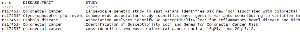
Maybe you are curious as to what other traits that same SNP might be associated with? Just reverse the criteria for omega and fatty acid strings. Here I also added the journal reference title, in case I wanted to read up more into these trait associations.

library(dplyr)
 select(output_data, rsid, DISEASE.TRAIT, STUDY) %>% 
 filter(!str_detect(tolower(DISEASE.TRAIT), "omega") & !str_detect(tolower(DISEASE.TRAIT), "fatty acid")) %>%
 distinct() %>%
 filter(rsid == "rs174537")

Now onto the second approach – this time, you don’t have a specific trait in mind. You’re more interested in discovering which traits have risk alleles that match the respective part of your genome. Please see all the above disclaimers. This is not remotely the same as saying which dreadful diseases you are going to get. But please stay away from this section if you are likely to be worried about seeing information that could even vaguely correspond to health concerns.

We already have our have_risk_allele_count field. If it’s 1 or 2 then you have some sort of match. So, the full list of your matches and the associated studies could be retrieved in a manner like this.

library(dplyr)
filter(output_data, have_risk_allele_count >= 1) %>%
 select(rsid, your_genotype = genotype, strongest_risk_allele = risk_allele_clean, DISEASE.TRAIT, STUDY )

Note that this list is likely to be long. Some risk alleles are very common in some populations, and remember that there may be many studies that relate to a single SNP, or many SNPs referred to by a single study. You might want to pop it in a nice DT Javascript DataTable to allow easy searching and sorting.

library(DT)
library(dplyr)

datatable(
 filter(output_data, have_risk_allele_count >= 1) %>%
 select(rsid, your_genotype = genotype, strongest_risk_allele = risk_allele_clean, DISEASE.TRAIT, STUDY )
)

results in something like:

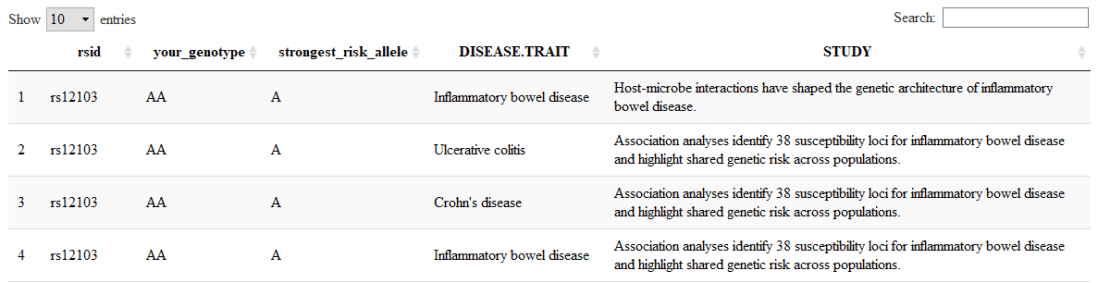
…which includes a handy search field at the top left of the output.

There are various other fields in the GWAS dataset you might consider using to filter down further. For example, you might be most interested in findings from studies that match your ethnicity, or occasions where you have risk alleles that are rare within the population. After all, we all like to think we’re special snowflakes, so if 95% of the general population have the risk allele for a trait, then that may be less interesting to an amateur genome explorer than one where you are in the lucky or unlucky 1%.

For the former, you might try searching within the INITIAL.SAMPLE.SIZE or REPLICATION.SAMPLE.SIZE fields, which has entries like: “272 Han Chinese ancestry individuals” or “1,180 European ancestry individuals from ~475 families”.

Similar to the caveats on searching the trait fields, one does need to be careful here if you’re looking for a comprehensive set of results. Some entries in the database have blanks in one of these fields, and others don’t specify ethnicities, having entries like “Up to 984 individuals”.

For the proportion of the studied population who had the risk allele, it’s the RISK.ALLELE.FREQUENCY field. Again, this can sometimes be blank or zero. But in theory, where it has a valid value, then, depending on the study design, you might find that lower frequencies are rarer traits.

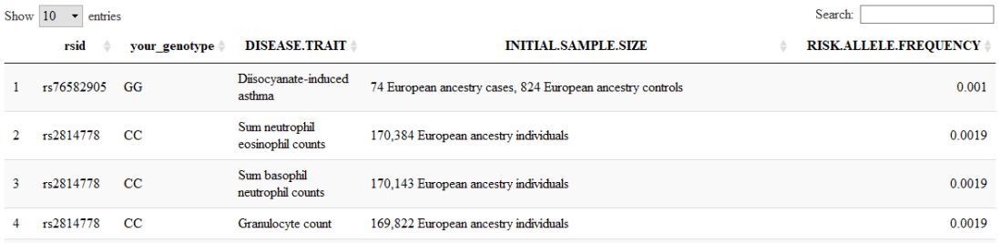
We can use dplyr‘s arrange and filter functions to sort do the above sort of narrowing-down. For example: what are the top 10 trait / study / SNP combinations you have the risk allele for that were explicitly studied within European folk, ordered by virtue of them having the lowest population frequencies reported in the study?

library(stringr)
library(dplyr)
head(
 filter(output_data,have_risk_allele_count > 0 & (str_detect(tolower(INITIAL.SAMPLE.SIZE), "european") | str_detect(tolower(REPLICATION.SAMPLE.SIZE), "european")) & (RISK.ALLELE.FREQUENCY > 0 & !is.na(RISK.ALLELE.FREQUENCY))) %>%
 arrange(RISK.ALLELE.FREQUENCY) %>%
 select(rsid, your_genotype = genotype, DISEASE.TRAIT, INITIAL.SAMPLE.SIZE,RISK.ALLELE.FREQUENCY)
 , 10)

 

 

Or perhaps you’d prefer to prioritise the order of the traits you have the risk allele for, for example, based on the number of entries in the GWAS database for that trait where the highest risk allele is one you have. You might argue that these could be some of the most reliably associated traits, in the sense that they would bias towards those that have so far been studied the most, at least within this database.

Let’s go graphical with this one, using the wonderful ggplot2 package.

library(dplyr)
library(ggplot2)

trait_entry_count <- group_by(output_data, DISEASE.TRAIT) %>%
 filter(have_risk_allele_count >= 1) %>%
 summarise(count_of_entries = n())

ggplot(filter(trait_entry_count, count_of_entries > 100), aes(x = reorder(DISEASE.TRAIT, count_of_entries, sum), y = count_of_entries)) +
 geom_col() +
 coord_flip() +
 theme_bw() +
 labs(title = "Which traits do you have the risk allele for\nthat have over 100 entries in the GWAS database?", y = "Count of entries", x = "Trait")

Now, as we’re counting combinations of studies and SNPs per trait here, this is obviously going to be somewhat self-fulfilling as some traits have been featured in way more studies than others. Likewise some traits may have been associated with many more SNPs than others. Also, recalling that many interesting traits seem to be related to a complex mix of SNPs, each of which may only have a tiny effect size, it might be that whilst you do have 10 of the risk alleles for condition X, you also don’t have the other 20 risk alleles that we discovered so far have an association (let alone the 100 weren’t even publish on yet and hence aren’t in this data!).

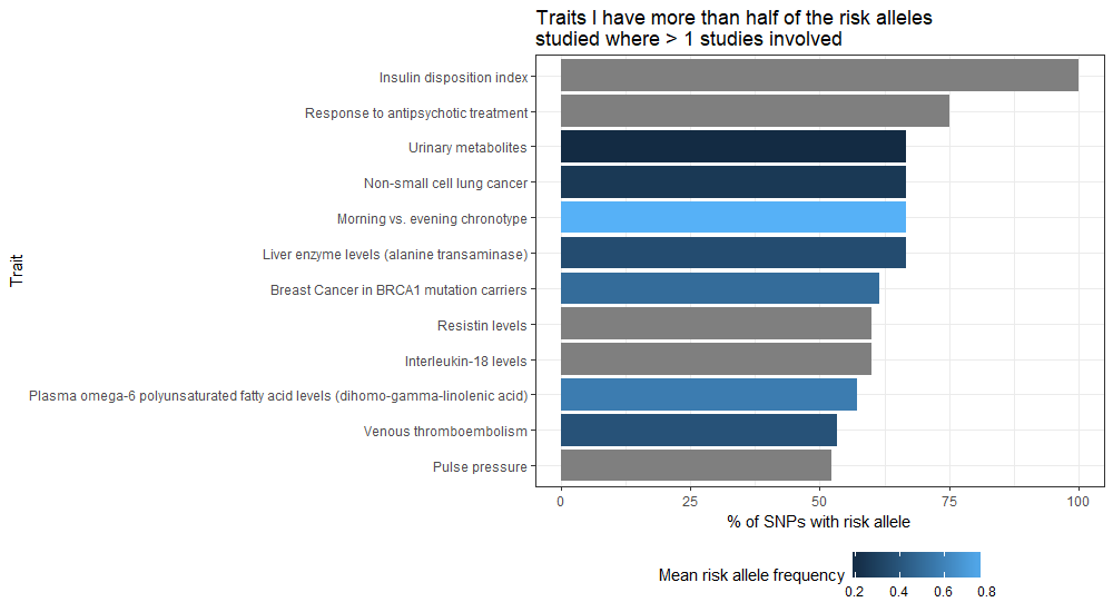
Maybe then we can sort our output in a different way. How about we count the number of distinct SNPs where you have the risk allele, and then express those as a proportion of the count of all the distinct SNPs for the given trait in the database, whether not you have the risk allele? This would let us say things such as, based (solely) on what in this database, you have 60% of the known risk alleles associated with this trait.

One thing noted in the data, both the 23andme genome data and the gwascat highest risk allele have unusual values in the allele fields – things like ?, -, R, D, I and some numbers based on the fact the “uncleaned” STRONGEST.SNP.RISK.ALLELE didn’t have a -A, -C, -G or -T at the end of the SNP it named. Some of these entries may be meaningful – for example the D and I in the 23andme data refer to deletes and insertions, but won’t match up with anything in the gwascat data. Others may be more messy or missing data, for example 23andme reports “–” if no genotype result was provided for a specific SNP call.

In order to avoid these inflating the proportion’s denominator we’ll just filter down so that we only consider entries where our gwascat-derived “risk_allele_clean” and  23andme-derived “my_allele_1” and “my_allele_2″ are all one of the standard A, C, G or T bases.

Let’s also colour code the results by the rarity of the SNP variant within the studied population. That might provide some insight to exactly what sort of special exception we are as an individual – although some of the GWAS data is missing that field and basic averaging won’t necessarily give the correct weighting, so this part is extra…”directional”.

You are no doubt getting bored with the sheer repetition of caveats here – but it is so important. Whilst these are refinements of sorts, they are simplistic and flawed and you should not even consider concluding something significant about your personal health without seeking professional advice here. This is fun only. Well, for for those of us who could ever possibly classify data as fun anyway.

Here we go, building it up one piece at a time for clarity of some kind:

library(dplyr)
library(ggplot2)

# Summarise proportion of SNPs for a given trait where you have a risk allele

trait_snp_proportion <-  filter(output_data, risk_allele_clean %in% c("C" ,"A", "G", "T") & my_allele_1 %in% c("C" ,"A", "G", "T") & my_allele_2 %in% c("C" ,"A", "G", "T") ) %>%
mutate(you_have_risk_allele = if_else(have_risk_allele_count >= 1, 1, 0)) %>%
 group_by(DISEASE.TRAIT, you_have_risk_allele) %>%
 summarise(count_of_snps = n_distinct(rsid)) %>%
 mutate(total_snps_for_trait = sum(count_of_snps), proportion_of_snps_for_trait = count_of_snps / sum(count_of_snps) * 100) %>%
 filter(you_have_risk_allele == 1) %>%
 arrange(desc(proportion_of_snps_for_trait)) %>%
 ungroup()

# Count the studies per trait in the database

trait_study_count <- filter(output_data, risk_allele_clean %in% c("C" ,"A", "G", "T") & my_allele_1 %in% c("C" ,"A", "G", "T") & my_allele_2 %in% c("C" ,"A", "G", "T") ) %>%
 group_by(DISEASE.TRAIT) %>%
 summarise(count_of_studies = n_distinct(PUBMEDID), mean_risk_allele_freq = mean(RISK.ALLELE.FREQUENCY))

# Merge the above together

trait_snp_proportion <- inner_join(trait_snp_proportion, trait_study_count, by = "DISEASE.TRAIT")

# Plot the traits where there were more than 2 studies and you have risk alleles for more than 70% of the SNPs studied

ggplot(filter(trait_snp_proportion, count_of_studies > 1 & proportion_of_snps_for_trait > 70), aes(x = reorder(DISEASE.TRAIT, proportion_of_snps_for_trait, sum), y = proportion_of_snps_for_trait, fill = mean_risk_allele_freq)) +
 geom_col() +
 coord_flip() +
 theme_bw() + 
 labs(title = "Traits I have more than half of the risk\nalleles studied where > 1 studies involved", 
 y = "% of SNPs with risk allele", x = "Trait", fill = "Mean risk allele frequency") +
 theme(legend.position="bottom")

 

Again, beware that the same sort of trait can be expressed in different ways within the data, in which case these entries are not combined. If you wanted to be more comprehensive regarding a specific trait, you might feel inclined to produce your own categorisation first and group by that – e.g. lumping anything BMI or Body Mass Index into your own BMI category via creating a new field.

Happy exploring!